4.2 Methods

superintronic is an R package used for estimating, representing, and visualising per-base coverage scores, that can then be flexibly summarised over factors within an experimental design and collapsed over regions of the genome using our companion package plyranges. The aspects of this combined workflow are summarised in Figure 4.2.

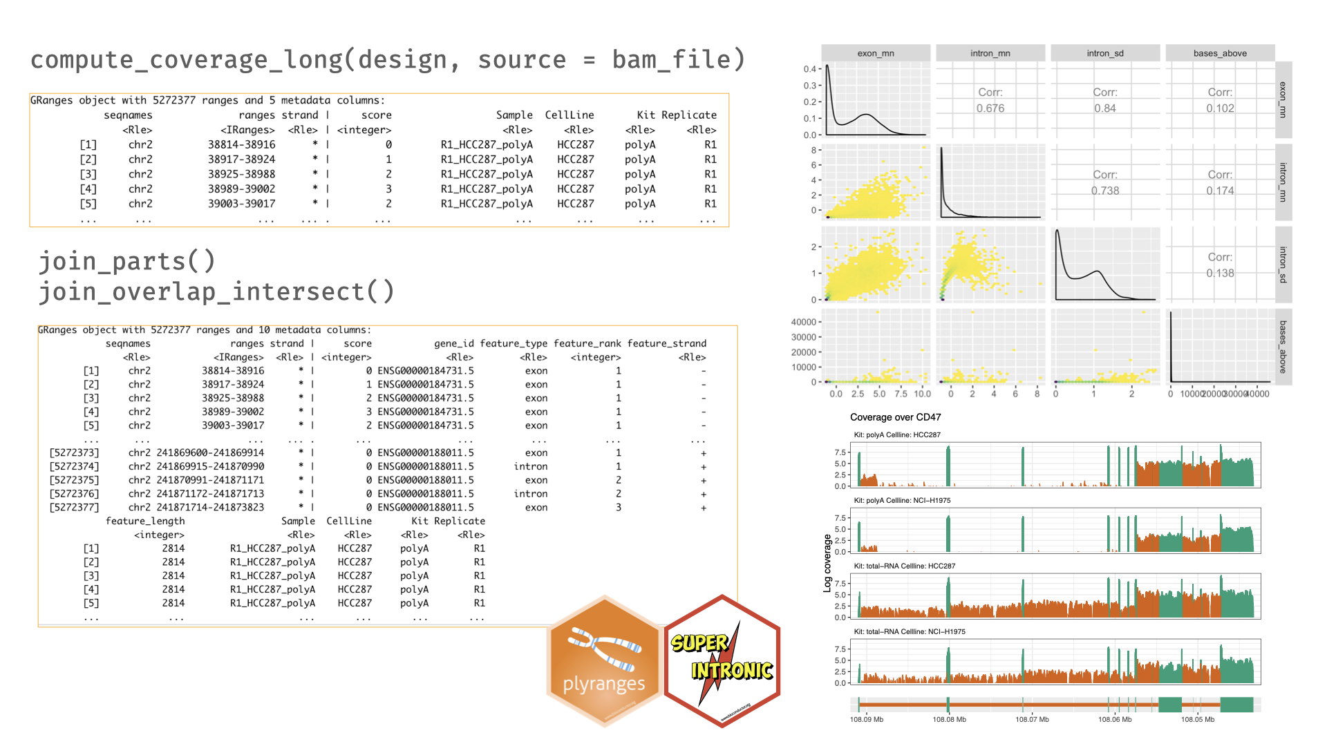
Figure 4.2: An overview of the superintronic and plyranges workflow. Coverage is estimated directly using the design matrix that contains a source column pointing to the locations of BAM files. The long-form representation is output as a GRanges object, and contains columns that were part of the design. Additional annotations are added with join functions, here we show the particular case of expanding the coverage GRanges to include exonic and intronic parts of a gene. This object can be further analysed using plyranges and our data descriptors approach, and then descriptors can be visualised as a scatter plot matrix with the GGally and ggplot2 packages (Schloerke et al. 2020; Wickham, Hadley 2016). Coverage traces can be directly generated with superintronic and collapsed over parts of the design matrix to identify differences between groups.

4.2.1 Representation of coverage estimation

The per base coverage score is estimated directly from one or more BAM files that represent the units within the experimental design, along with an optional experimental design table that is returns a long-form tidy GRanges data structure. The coverage estimation is computed via the Rsamtools package, and users have the ability to estimate coverage in parallel and drop regions in the genome where there is no coverage (Morgan et al. 2020; Lawrence et al. 2013b). This representation is tidy, since each row of the resulting GRanges data structure corresponds to position(s) within a given sample with a given coverage score alongside any variables such as biological group. While the long-form representation repeats the same information for a sample within the design, the size of the resulting GRanges in memory can be compressed using run-length encoding for any categorical variable, which is a form of data compression where “runs” of a vector are stored rather than their values. For example, the character vector of letters “a”, and “b” is shortened so successive values are stored as a single value with their lengths:

#>  [1] "b" "a" "b" "b" "a" "a" "b" "a" "a" "a"

#> character-Rle of length 10 with 6 runs
#>   Lengths:   1   1   2   2   1   3
#>   Values : "b" "a" "b" "a" "b" "a"

This representation is memory efficient: at worst it will be the same size as the input, and at best reduce the size by a factor corresponding to the largest run. The allows us to easily transform the coverage scores and integrate annotations using the plyranges grammar, and visualise traces using ggplot2 (Wickham, Hadley 2016).

4.2.2 Integration of external annotations

External reference annotations, perhaps transcripts or exons, can be coerced to GRanges objects, are incorporated into the coverage GRanges by taking the intersection of the annotation with the GRanges using an overlap intersect join from the plyranges software. The resulting intersection will now contain the per base coverage that are overlapped the genomic features in the annotation, along side any metadata about the features themselves. Since our main workflow interest is in discovering coverage traces with IR profiles, superintronic provides some syntactic sugar for unravelling gene annotations into their exonic and intronic parts, and intersecting them with a coverage GRanges. Split reads that cross the boundaries of exon and intron parts are counted towards both unless filtered beforehand.

4.2.3 Discovery of regions of interest via ‘data descriptors’

Once the coverage GRanges has reference genomic features, data descriptors can be computed via collecting summary statistics across the factors of the experimental design and features of interest. This can be achieved using plyranges directly by first grouping across variables of interest, computing descriptors defined by superintronic and then pivoting the results into a wide form table for additional processing or visualisation. There are many descriptors defined by superintronic that are weighted statistics (as we have to account for the number of bases covered, or the width of the range) of the coverage score, such as the mean and standard deviation. There are also descriptors that can be used to find the number of times the coverage trace is above a certain number of bases or score. To find coverage traces that have unusual descriptors, the descriptors can be visualised directly as a scatter plot matrix. After that thresholds can be applied to filter the genomic features that had extreme descriptors on the coverage GRanges, and the traces can be visualised. By default superintronic displays coverage traces oriented from the 5’ to 3’ end of the gene, with the view_coverage() function. Traces can be highlighted according to a genomic feature of interest, figures in this chapter have orange areas corresponding to intronic parts of the gene, while dark green areas referring to exonic parts.