3.3 Model assays
3.3.1 RNA-seq differential gene expression analysis
We can easily run a differential expression analysis with DESeq2 using the following code chunks (Love, Huber, and Anders 2014). The design formula indicates that we want to control for the donor baselines (line) and test for differences in gene expression on the condition. For a more comprehensive discussion of DE workflows in Bioconductor see Love et al. (2016) and Law et al. (2018).
library(DESeq2)
dds <- DESeqDataSet(gse, ~line + condition)
# filter out lowly expressed genes
# at least 10 counts in at least 6 samples
keep <- rowSums(counts(dds) >= 10) >= 6
dds <- dds[keep,]
The model is fit with the following line of code:
Below we set the contrast on the condition variable, indicating we are estimating the \(\log_2\) fold change (LFC) of IFNg stimulated cell lines against naive cell lines. We are interested in LFC greater than 1 at a nominal false discovery rate (FDR) of 1%.
The results() function extracts a summary of the DE analysis: in this case for each gene we have the LFC comparing the two cell lines, the Wald test statistic of LFC from the fitted negative binomial GLM, and associated p-value and corrected p-value accounting for the FDR. To see the results of the expression analysis, we can generate a summary table and a mean-abundance (MA) plot (Dudoit et al. 2002):
#>
#> out of 17806 with nonzero total read count
#> adjusted p-value < 0.01
#> LFC > 1.00 (up)    : 502, 2.8%
#> LFC < -1.00 (down) : 247, 1.4%
#> outliers [1]       : 0, 0%
#> low counts [2]     : 0, 0%
#> (mean count < 3)
#> [1] see 'cooksCutoff' argument of ?results
#> [2] see 'independentFiltering' argument of ?results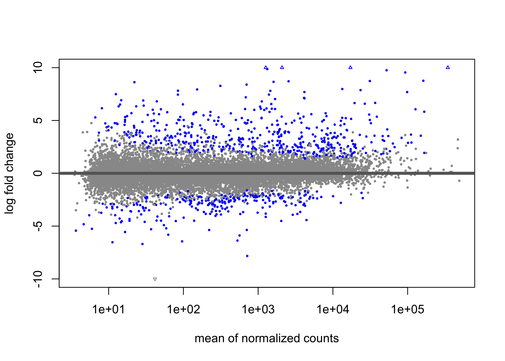
Figure 3.3: Visualization of DESeq2 results as an “MA plot”. Genes that have an adjusted p-value below 0.01 are colored blue.In this case the LFC between conditions is shown on the y-axis, while the average normalised gene counts across all conditions are shown on the x-axis. The assumption of an RNA-seq analysis that most genes are not DE, so most genes are scattered about zero on the y-axis while genes that have evidence of DE are far from the zero baseline. The x-axis gives a sense of the total expression of the gene.
We now output the results as a GRanges object, and due to the conventions of plyranges, we construct a new column called gene_id from the row names of the results. Each row now contains the genomic region ( seqnames, start, end, strand) along with corresponding metadata columns (the gene_id and the results of the test). Note that tximeta has correctly identified the reference genome as “hg38”, and this has also been added to the GRanges along the results columns. This kind of book-keeping is vital once overlap operations are performed to ensure that plyranges is not comparing across incompatible genomes.
suppressPackageStartupMessages(library(plyranges))
de_genes <- results(dds,
                    contrast=c("condition","IFNg","naive"),
                    lfcThreshold=1,
                    format="GRanges") %>%
  names_to_column("gene_id")
de_genes
#> GRanges object with 17806 ranges and 7 metadata columns:
#> seqnames ranges strand | gene_id baseMean
#> <Rle> <IRanges> <Rle> | <character> <numeric>
#> [1] chrX 100627109-100639991 - | ENSG00000000003.14 171.571
#> [2] chr20 50934867-50958555 - | ENSG00000000419.12 967.751
#> [3] chr1 169849631-169894267 - | ENSG00000000457.13 682.433
#> [4] chr1 169662007-169854080 + | ENSG00000000460.16 262.963
#> [5] chr1 27612064-27635277 - | ENSG00000000938.12 2660.102
#> ... ... ... ... . ... ...
#> [17802] chr10 84167228-84172093 - | ENSG00000285972.1 10.04746
#> [17803] chr6 63572012-63583587 + | ENSG00000285976.1 4586.34617
#> [17804] chr16 57177349-57181390 + | ENSG00000285979.1 14.29653
#> [17805] chr8 103398658-103501895 - | ENSG00000285982.1 27.76296
#> [17806] chr10 12563151-12567351 + | ENSG00000285994.1 6.60409
#> log2FoldChange lfcSE stat pvalue padj
#> <numeric> <numeric> <numeric> <numeric> <numeric>
#> [1] -0.2822450 0.3005710 0.00000 1.0000000 1.000000
#> [2] 0.0391223 0.0859708 0.00000 1.0000000 1.000000
#> [3] 1.2846179 0.1969067 1.44545 0.1483329 1.000000
#> [4] -1.4718762 0.2186916 -2.15772 0.0309493 0.409728
#> [5] 0.6754781 0.2360530 0.00000 1.0000000 1.000000
#> ... ... ... ... ... ...
#> [17802] 0.5484518 0.444319 0 1 1
#> [17803] -0.0339296 0.188005 0 1 1
#> [17804] 0.3123477 0.522700 0 1 1
#> [17805] 0.9945187 1.582373 0 1 1
#> [17806] 0.2539975 0.595751 0 1 1
#> -------
#> seqinfo: 25 sequences (1 circular) from hg38 genomeFrom this, we can restrict the results to those that meet our FDR threshold and select (and rename) the metadata columns we are interested in:
de_genes <- de_genes %>%
  filter(padj < 0.01) %>%
  select(
    gene_id,
    de_log2FC = log2FoldChange,
    de_padj = padj
  )
We now wish to extract genes for which there is evidence that the LFC is not
large. We perform this test by specifying an LFC threshold and an alternative
hypothesis (altHypothesis) that the LFC is less than the threshold in
absolute value. In this case, the p-values are taken as maximum of the upper and lower Wald tests under the hypothesis absolute value of the estimated LFC is lower than the threshold. To visualize the result of this test, you can run results
without format="GRanges", and pass this object to plotMA() as before. We
label these genes as other_genes and later as “non-DE genes”, for comparison
with our de_genes set.
3.3.2 ATAC-seq peak differential abundance analysis
The following section describes the process we have used for generating a GRanges object of differential peaks from the ATAC-seq data in Alasoo et al. (2018). The code chunks for the remainder of this section are optional.
For assessing differential accessibility, we run limma (Smyth 2004), and generate the a summary of LFCs and adjusted p-values for the peaks:
library(limma)
design <- model.matrix(~donor + condition, colData(atac))
fit <- lmFit(assay(atac), design)
fit <- eBayes(fit)
idx <- which(colnames(fit$coefficients) == "conditionIFNg")
tt <- topTable(fit, coef=idx, sort.by="none", n=nrow(atac))
We now take the rowRanges() of the SummarizedExperiment and attach the LFCs
and adjusted p-values from limma, so that we can consider the overlap with
differential expression. Note that we set the genome build to “hg38” and
restyle the chromosome information to use the “UCSC” style (e.g. “chr1”,
“chr2”, etc.). Again, we know the genome build from the Zenodo entry for the
ATAC-seq data.
atac_peaks <- rowRanges(atac) %>%
  remove_names() %>%
  mutate(
    da_log2FC = tt$logFC,
    da_padj = tt$adj.P.Val
  ) %>%
  set_genome_info(genome = "hg38")

seqlevelsStyle(atac_peaks) <- "UCSC"
The final GRanges object containing the DA peaks is included in the fluentGenomics and can be loaded as follows:
#> GRanges object with 296220 ranges and 3 metadata columns:
#>            seqnames              ranges strand |          peak_id da_log2FC
#>               <Rle>           <IRanges>  <Rle> |      <character> <numeric>
#>        [1]     chr1          9979-10668      * |      ATAC_peak_1  0.266185
#>        [2]     chr1         10939-11473      * |      ATAC_peak_2  0.322177
#>        [3]     chr1         15505-15729      * |      ATAC_peak_3 -0.574160
#>        [4]     chr1         21148-21481      * |      ATAC_peak_4 -1.147066
#>        [5]     chr1         21864-22067      * |      ATAC_peak_5 -0.896143
#>        ...      ...                 ...    ... .              ...       ...
#>   [296216]     chrX 155896572-155896835      * | ATAC_peak_296216 -0.834629
#>   [296217]     chrX 155958507-155958646      * | ATAC_peak_296217 -0.147537
#>   [296218]     chrX 156016760-156016975      * | ATAC_peak_296218 -0.609732
#>   [296219]     chrX 156028551-156029422      * | ATAC_peak_296219 -0.347678
#>   [296220]     chrX 156030135-156030785      * | ATAC_peak_296220  0.492442
#>                da_padj
#>              <numeric>
#>        [1] 9.10673e-05
#>        [2] 2.03435e-05
#>        [3] 3.41708e-08
#>        [4] 8.22299e-26
#>        [5] 4.79453e-11
#>        ...         ...
#>   [296216] 1.33546e-11
#>   [296217] 3.13015e-01
#>   [296218] 3.62339e-09
#>   [296219] 6.94823e-06
#>   [296220] 7.07664e-13
#>   -------
#>   seqinfo: 23 sequences from hg38 genome; no seqlengths