2.2 Results
2.2.1 Genomic Relational Algebra
2.2.1.1 Data Model
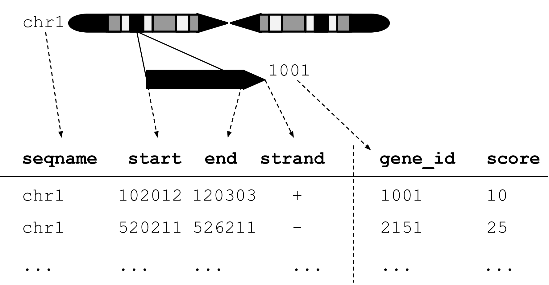
Figure 2.1: An illustration of the GRanges data model for a sample from an RNA-seq experiment. The core components of the data model include a seqname column (representing the chromosome), a ranges column which consists of start and end coordinates for a genomic region, and a strand identifier (either positive, negative, or unstranded). Metadata are included as columns to the right of the dotted line as annotations (gene_id) or range level covariates (score).
The plyranges DSL is built on the core Bioconductor data structure GRanges, which is a constrained table, with fixed columns for the chromosome, start and end coordinates, and the strand, along with an arbitrary set of additional columns, consisting of measurements or metadata specific to the data type or experiment (Figure 2.1). GRanges balances flexibility with formal constraints, so that it is applicable to virtually any genomic workflow, while also being semantically rich enough to support high-level operations on genomic ranges. As a core data structure, GRanges enables interoperability between plyranges and the rest of Bioconductor. Adhering to a single data structure simplifies the API and makes it easier to learn and understand, in part because operations become endomorphic, i.e., they return the same type as their input.
GRanges follow the intuitive tidy data pattern: it is a rectangular table corresponding to a single biological context. Each row contains a single observation and each column is a variable describing the observations. GRanges specializes the tidy pattern in that the observations always pertain to some genomic feature, but it largely remains compatible with the general relational operations defined by dplyr. Thus, we define our algebra as an extension of the dplyr algebra, and borrow its syntax conventions and design principles.
2.2.1.2 Algebraic operations
The plyranges DSL defines an expressive algebra for performing genomic operations with and between GRanges objects (see table ). The grammar includes several classes of operation that cover most use cases in genomics data analysis. There are range arithmetic operators, such as for resizing ranges or finding their intersection, and operators for merging, filtering and aggregating by range-specific notions like overlap and proximity.
Arithmetic operations transform range coordinates, as defined by their start, end and width. The three dimensions are mutually dependent and partially redundant, so direct manipulation of them is problematic. For example, changing the width column needs to change either the start, end or both to preserve integrity of the object. We introduce the anchor modifier to disambiguate these adjustments. Supported anchor points include the start, end and midpoint, as well as the 3’ and 5’ ends for strand-directed ranges. For example, if we anchor the start, then setting the width will adjust the end while leaving the start stationary.
The algebra also defines conveniences for relative coordinate
adjustments: shift (unanchored adjustment to both start and end) and
stretch (anchored adjustment of width). We can perform any relative
adjustment by some combination of those two operations. The stretch
operation requires an anchor and assumes the midpoint by
default. Since shift is unanchored, the user specifies a suffix for
indicating the direction: left/right or, for stranded features,
upstream/downstream. For example, shift_right() shifts a range to the
right.
The flank operation generates new ranges that are adjacent to existing ones. This is useful, for example, when generating upstream promoter regions for genes. Analogous to shift, a suffix indicates the side of the input range to flank.
As with other genomic grammars, we define set operations that treat
ranges as sets of integers, including intersect, union,
difference, and complement. There are two sets of these: parallel
and merging. For example, the parallel intersection (x %intersect% y) finds the
intersecting range between xi and yi for i in 1…n, where n
is the length of both x and y. In contrast, the merging
intersection ( intersect_ranges(x, y)) returns a new set of disjoint
ranges representing wherever there was overlap between a range in x
and a range in y. Finding the parallel union will fail when two ranges
have a gap, so we introduce a span() operator that takes the union
while filling any gap. The complement() operation is unique in that it
is unary. It finds the regions not covered by any of the ranges in a
single set. Closely related is the between() parallel operation, which
finds the gap separating xi and yi. The binary operations are
callable from within arithmetic, restriction and aggregation
expressions.
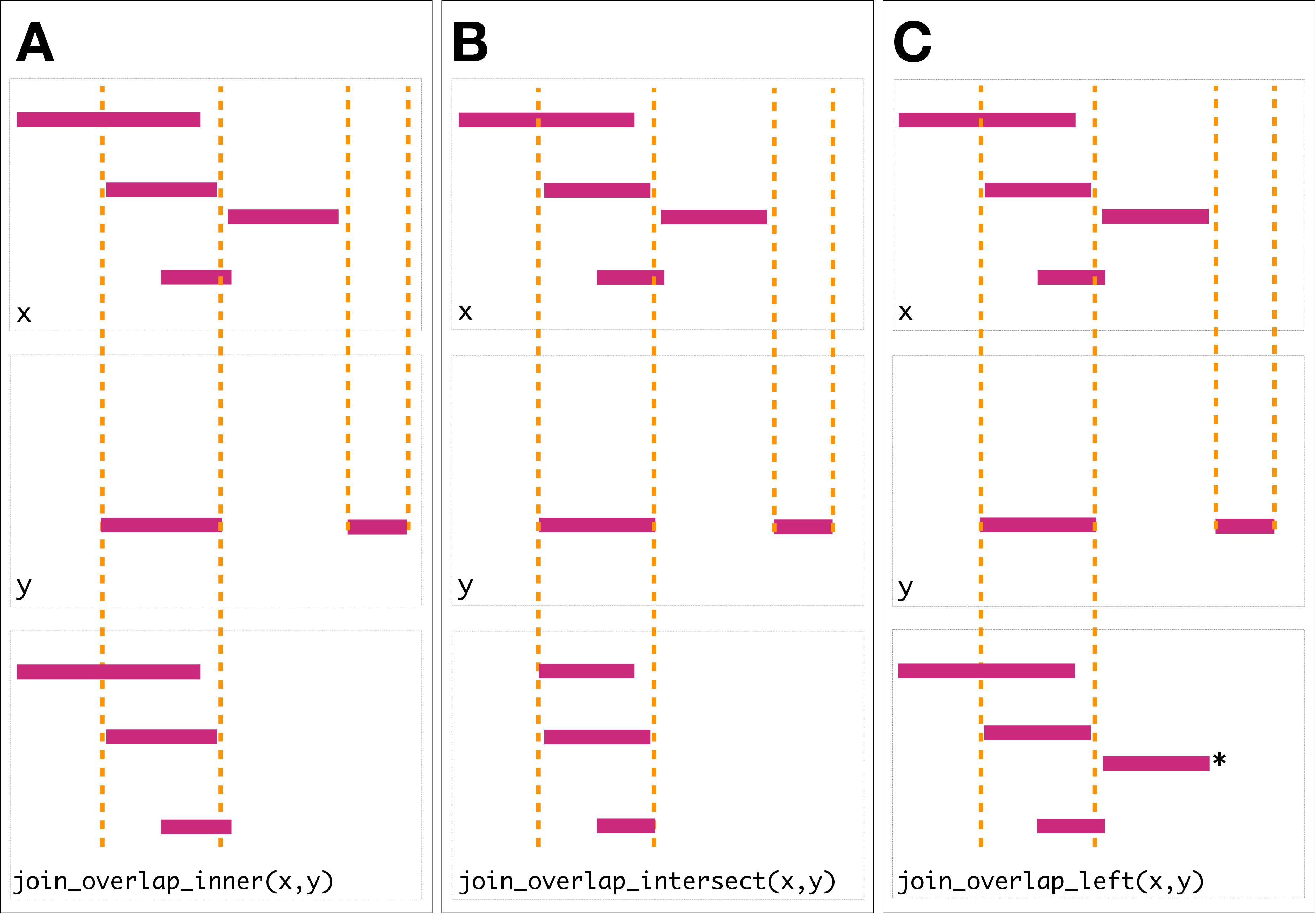
Figure 2.2: Illustration of the three overlap join operators. Each join takes two GRanges objects, and as input. A ‘Hits’ object for the join is computed which consists of two components. The first component contains the indices of the ranges in that have been overlapped (the rectangles of that cross the orange lines). The second component consists of the indices of the ranges in that overlap the ranges in . In this case a range in overlaps the ranges in three times, so the index is repeated three times. The resulting ‘Hits’ object is used to modify by where it was ‘hit’ by and merge all metadata columns from and based on the indices contained in the ‘Hits’ object. This procedure is applied generally in the DSL for both overlap and nearest neighbor operations. The join semantics alter what is returned: : for an join the ranges that are overlapped by are returned. The returned ranges also include the metadata from the range that overlapped the three ranges. An join is identical to an inner join except that the intersection is taken between the overlapped ranges and the ranges. For the join all ranges are returned regardless of whether they are overlapped by . In this case the third range (rectangle with the asterisk next to it) of the join would have missing values on metadata columns that came from .
To support merging, our algebra recasts finding overlaps or nearest neighbors between two genomic regions as variants of the relational join operator. A join acts on two GRanges objects: x and y. The join operator is relational in the sense that metadata from the x and y ranges are retained in the joined range. All join operators in the plyranges DSL generate a set of hits based on overlap or proximity of ranges and use those hits to merge the two datasets in different ways. There are four supported matching algorithms: overlap, nearest, precede, and follow (Figure 2.2). We can further restrict the matching by whether the query is completely within the subject, and adding the directed suffix ensures that matching ranges have the same direction (strand).
For merging based on the hits, we have three modes: inner, intersect and left. The inner overlap join is similar to the conventional inner join in that there is a row in the result for every match. A major difference is that the matching is not by identity, so we have to choose one of the ranges from each pair. We always choose the left range. The intersect join uses the intersection instead of the left range. Finally, the overlap left join is akin to left outer join in Codd’s relational algebra: it performs an overlap inner join but also returns all x ranges that are not hit by the y ranges.
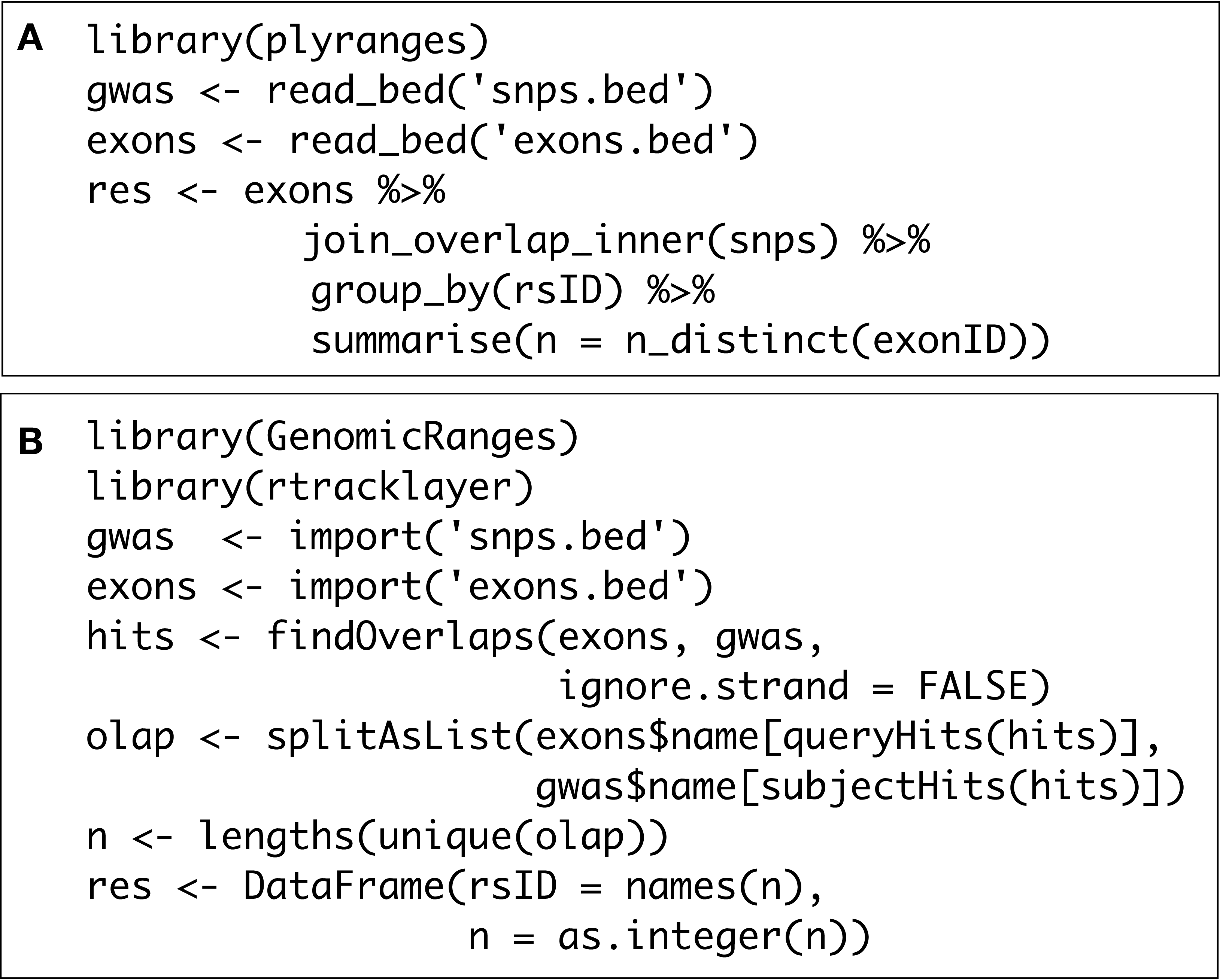
Figure 2.3: Idiomatic code examples for () and () illustrating an overlap and aggregate operation that returns the same result. In each example, we have two BED files consisting of SNPs that are genome-wide association study (GWAS) hits and reference exons. Each code block counts for each SNP the number of distinct exons it overlaps. The code achieves this with an overlap join followed by partitioning and aggregation. Strand is ignored by default here. The code achieves this using the Hits and List classes and their methods.
Since the GRanges object is a tabular data structure, our grammar includes
operators to filter, sort and aggregate by columns in a GRanges. These
operations can be performed over partitions formed
using the group_by() modifier. Together with our algebra for arithmetic and
merging, these operations conform to the semantics and syntax of the
dplyr grammar. Consequently, plyranges code is generally more compact
than the equivalent GenomicRanges code (Figure 2.3).
2.2.2 Developing workflows with plyranges
Here we provide illustrative examples of using the plyranges DSL to show how our grammar could be integrated into genomic data workflows. As we construct the workflows we show the data output intermittently to assist the reader in understanding the pipeline steps. The workflows highlight how interoperability with existing Bioconductor infrastructure, enables easy access to public datasets and methods for analysis and visualization.
2.2.2.1 Peak Finding
In the workflow of ChIP-seq data analysis, we are interested in finding peaks from islands of coverage over chromosome. Here we will use plyranges to call peaks from islands of coverage above 8 then plot the region surrounding the tallest peak.
Using plyranges and the Bioconductor package AnnotationHub (Morgan 2017) we can download and read BigWig files from ChIP-Seq experiments from the Human Epigenome Roadmap project (Roadmap Epigenomics Consortium et al. 2015). Here we analyse a BigWig file corresponding to H3 lysine 27 trimethylation (H3K27Me3) of primary T CD8+ memory cells from peripheral blood, focussing on coverage islands over chromosome 10.
First, we extract the genome information from the BigWig file and filter to get the range for chromosome 10. This range will be used as a filter when reading the file.
Then we read the BigWig file only extracting scores if they overlap chromosome 10. We also add the genome build information to the resulting ranges. This book-keeping is good practice as it ensures the integrity of any downstream operations such as finding overlaps.
chr10_scores <- bw_file %>%
  read_bigwig(overlap_ranges = chr10_ranges) %>%
  set_genome_info(genome = "hg19")
chr10_scores
#> GRanges object with 5789841 ranges and 1 metadata column:
#> seqnames ranges strand | score
#> <Rle> <IRanges> <Rle> | <numeric>
#> [1] chr10 1-60602 * | 0.04228
#> [2] chr10 60603-60781 * | 0.16324
#> [3] chr10 60782-60816 * | 0.37214
#> [4] chr10 60817-60995 * | 0.16324
#> [5] chr10 60996-61625 * | 0.04228
#> ... ... ... ... . ...
#> [5789837] chr10 135524723-135524734 * | 0.14432
#> [5789838] chr10 135524735-135524775 * | 0.25023
#> [5789839] chr10 135524776-135524784 * | 0.42779
#> [5789840] chr10 135524785-135524806 * | 0.73002
#> [5789841] chr10 135524807-135524837 * | 1.03103
#> -------
#> seqinfo: 25 sequences from hg19 genomeWe then filter for regions with a coverage score greater than 8, and following
this reduce individual runs to ranges representing the islands of coverage.
This is achieved with the reduce_ranges() function, which allows a summary
to be computed over each island: in this case we take the maximum of
the scores to find the coverage peaks over chromosome 10.
#> GRanges object with 1085 ranges and 1 metadata column:
#>          seqnames              ranges strand |     score
#>             <Rle>           <IRanges>  <Rle> | <numeric>
#>      [1]    chr10     1299144-1299370      * |  13.22640
#>      [2]    chr10     1778600-1778616      * |   8.20512
#>      [3]    chr10     4613068-4613078      * |   8.76027
#>      [4]    chr10     4613081-4613084      * |   8.43660
#>      [5]    chr10             4613086      * |   8.11508
#>      ...      ...                 ...    ... .       ...
#>   [1081]    chr10 135344482-135344488      * |   9.23238
#>   [1082]    chr10 135344558-135344661      * |  11.84341
#>   [1083]    chr10 135344663-135344665      * |   8.26966
#>   [1084]    chr10 135344670-135344674      * |   8.26966
#>   [1085]    chr10 135345440-135345441      * |   8.26966
#>   -------
#>   seqinfo: 25 sequences from hg19 genome
Returning to the GRanges object containing normalized coverage scores, we filter to find the coordinates of the peak containing the maximum coverage score. We can then find a 5000 nt region centered around the maximum position by anchoring and modifying the width.
Finally, the overlap inner join is used to restrict the chromosome 10 coverage islands, to the islands that are contained in the 5000nt region that surrounds the max peak (Figure 2.4).
#> GRanges object with 890 ranges and 2 metadata columns:
#>         seqnames            ranges strand |   score.x   score.y
#>            <Rle>         <IRanges>  <Rle> | <numeric> <numeric>
#>     [1]    chr10 21805891-21805988      * |   0.02066   29.9573
#>     [2]    chr10 21805989-21806000      * |   0.02112   29.9573
#>     [3]    chr10 21806001-21806044      * |   0.02207   29.9573
#>     [4]    chr10 21806045-21806049      * |   0.02159   29.9573
#>     [5]    chr10 21806050-21806081      * |   0.02112   29.9573
#>     ...      ...               ...    ... .       ...       ...
#>   [886]    chr10          21810878      * |   5.24952   29.9573
#>   [887]    chr10          21810879      * |   5.83534   29.9573
#>   [888]    chr10 21810880-21810884      * |   6.44268   29.9573
#>   [889]    chr10 21810885-21810895      * |   7.07055   29.9573
#>   [890]    chr10 21810896-21810911      * |   6.44268   29.9573
#>   -------
#>   seqinfo: 25 sequences from hg19 genome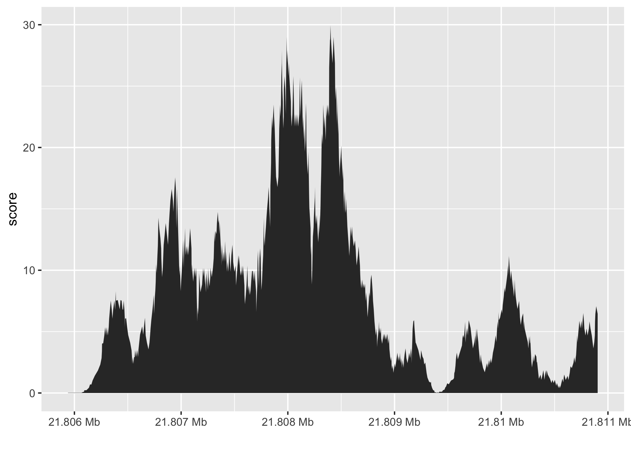
Figure 2.4: The final result of the plyranges operations to find a 5000nt region surrounding the peak of normalised coverage scores over chromosome 10, displayed as a density plot.
2.2.2.2 Computing Windowed Statistics
Another common operation in genomics data analysis is to compute data
summaries over genomic windows. In plyranges this can be achieved
via the group_by_overlaps() operator. We bin and count and
find the average GC content of reads from a
H3K27Me3 ChIP-seq experiment by the Human Epigenome Roadmap
Consortium.
We can directly obtain the genome information from the header of the BAM file: in this case the reads were aligned to the hg19 genome build and there are no reads overlapping the mitochondrial genome.
Next we only read in alignments that overlap the genomic locations
we are interested in and select the query sequence. Note that
the reading of the BAM file is deferred: only alignments that pass the filter
are loaded into memory. We can add another column representing the GC proportion
for each alignment using the letterFrequency() function from the Biostrings
package (Pagès et al. 2018). After computing the GC proportion as the score
column, we drop all other columns in the GRanges object.
alignments <- bam %>%
  filter_by_overlaps(locations) %>%
  select(seq) %>%
  mutate(
    score = as.numeric(letterFrequency(seq, "GC", as.prob = TRUE))
  ) %>%
  select(score)
alignments
#> GRanges object with 8275595 ranges and 1 metadata column:
#> seqnames ranges strand | score
#> <Rle> <IRanges> <Rle> | <numeric>
#> [1] chr10 50044-50119 - | 0.276316
#> [2] chr10 50050-50119 + | 0.250000
#> [3] chr10 50141-50213 - | 0.447368
#> [4] chr10 50203-50278 + | 0.263158
#> [5] chr10 50616-50690 + | 0.276316
#> ... ... ... ... . ...
#> [8275591] chrY 57772745-57772805 - | 0.513158
#> [8275592] chrY 57772751-57772800 + | 0.526316
#> [8275593] chrY 57772767-57772820 + | 0.565789
#> [8275594] chrY 57772812-57772845 + | 0.250000
#> [8275595] chrY 57772858-57772912 + | 0.592105
#> -------
#> seqinfo: 24 sequences from an unspecified genomeFinally, we create 10000nt tiles over the genome and compute the number of reads and average GC content over all reads that fall within each tile using an overlap join and merging endpoints.
bins <- locations %>%
  tile_ranges(width = 10000L)

alignments_summary <- bins %>%
  join_overlap_inner(alignments) %>%
  disjoin_ranges(n = n(), avg_gc = mean(score))
alignments_summary
#> GRanges object with 286030 ranges and 2 metadata columns:
#> seqnames ranges strand | n avg_gc
#> <Rle> <IRanges> <Rle> | <integer> <numeric>
#> [1] chr10 49999-59997 * | 88 0.369019
#> [2] chr10 59998-69997 * | 65 0.434211
#> [3] chr10 69998-79996 * | 56 0.386513
#> [4] chr10 79997-89996 * | 71 0.512973
#> [5] chr10 89997-99996 * | 64 0.387747
#> ... ... ... ... . ... ...
#> [286026] chrY 57722961-57732958 * | 36 0.468202
#> [286027] chrY 57732959-57742957 * | 38 0.469529
#> [286028] chrY 57742958-57752956 * | 38 0.542936
#> [286029] chrY 57752957-57762955 * | 42 0.510652
#> [286030] chrY 57762956-57772954 * | 504 0.526942
#> -------
#> seqinfo: 24 sequences from an unspecified genome; no seqlengths2.2.2.3 Quality Control Metrics
We have created a GRanges object from genotyping performed on the H1 cell line, consisting of approximately two million single nucleotide polymorphisms (SNPs) and short insertion/deletions (indels). The GRanges object consists of 7 columns, relating to the alleles of a SNP or indel, the B-allele frequency, log relative intensity of the probes, GC content score over a probe, and the name of the probe. We can use this information to compute the transition-transversion ratio, a quality control metric, within each chromosome in GRanges object.
First we filter out the indels and mitochondrial variants. Then we create a logical vector corresponding to whether there is a transition event.
h1_snp_array <- h1_snp_array %>%
  filter(!(ref %in% c("I", "D")), seqnames != "M") %>%
  mutate(transition = (ref %in% c("A", "G") & alt %in% c("G","A"))|
                      (ref %in% c("C","T") & alt %in% c("T", "C")))
We then compute the transition-transversion ratio over each chromosome using
group_by() in combination with summarize() (Figure 2.5).
ti_tv_results <- h1_snp_array %>%
  group_by(seqnames) %>%
  summarize(n_snps = n(),
            ti_tv = sum(transition) / sum(!transition))
ti_tv_results
#> DataFrame with 24 rows and 3 columns
#> seqnames n_snps ti_tv
#> <Rle> <integer> <numeric>
#> 1 Y 2226 1.43812
#> 2 6 154246 3.32013
#> 3 13 83736 3.40669
#> 4 10 120035 3.49401
#> 5 4 153243 3.29529
#> ... ... ... ...
#> 20 16 77538 3.19828
#> 21 12 113208 3.47852
#> 22 20 57073 3.71210
#> 23 21 32349 3.50480
#> 24 X 55495 3.58220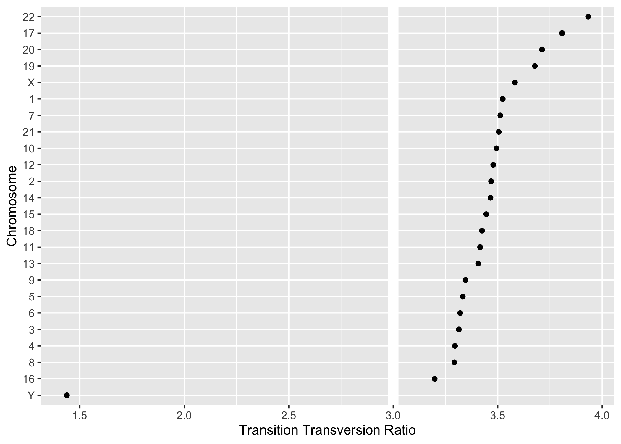
Figure 2.5: The final result of computing quality control metrics over the SNP array data with plyranges, displayed as a dot plot. Chromosomes are ordered by their estimated transition-transversion ratio. A white reference line is drawn at the expected ratio for a human exome."