3.4 Integrate ranges
3.4.1 Finding overlaps with plyranges
We have already used plyranges a number of times above, to filter(),
mutate(), and select() on GRanges objects, as well as ensuring the correct
genome annotation and style has been used. The plyranges package provides a
grammar for performing transformations of genomic data (Lee, Cook, and Lawrence 2019). Computations
resulting from compositions of plyranges “verbs” are performed using
underlying, highly optimized range operations in the GenomicRanges package
(Lawrence et al. 2013b).
For the overlap analysis, we filter the annotated peaks to have a nominal FDR bound of 1%.
We now have GRanges objects that contain DE genes, genes without strong signal of DE, and DA peaks. We are ready to answer the question: is there an enrichment of DA ATAC-seq peaks in the vicinity of DE genes compared to genes without sufficient DE signal?
3.4.2 Down sampling non-differentially expressed genes
As plyranges is built on top of dplyr, it implements methods for many of
its verbs for GRanges objects. Here we can use slice() to randomly sample the
rows of the other_genes. The sample.int() function will generate random
samples of size equal to the number of DE-genes from the number of rows in
other_genes:
#> GRanges object with 749 ranges and 3 metadata columns:
#>         seqnames              ranges strand |            gene_id  de_log2FC
#>            <Rle>           <IRanges>  <Rle> |        <character>  <numeric>
#>     [1]    chr12   57520710-57530148      + | ENSG00000166987.14 -0.1731698
#>     [2]    chr22   41459717-41468725      - |  ENSG00000100410.7 -0.0364158
#>     [3]     chr9   34329506-34343713      + | ENSG00000164978.17  0.0484335
#>     [4]     chr1   27830778-27851676      + | ENSG00000117751.17 -0.1340895
#>     [5]    chr12   50129306-50167533      - | ENSG00000139624.12  0.3348782
#>     ...      ...                 ...    ... .                ...        ...
#>   [745]    chr22   19175575-19178830      - |  ENSG00000100075.9 -0.0431335
#>   [746]     chr9 132375548-132406851      - | ENSG00000125482.12 -0.3859562
#>   [747]    chr20   17941597-17968980      - | ENSG00000089006.16 -0.3609427
#>   [748]     chr9 122940833-123104866      + | ENSG00000011454.16  0.0981684
#>   [749]    chr18   58862600-58986480      + | ENSG00000074657.13  0.2913740
#>             de_padj
#>           <numeric>
#>     [1] 1.13014e-12
#>     [2] 1.19682e-17
#>     [3] 1.45952e-18
#>     [4] 2.46329e-23
#>     [5] 1.06269e-14
#>     ...         ...
#>   [745] 5.97384e-15
#>   [746] 4.56944e-14
#>   [747] 3.85372e-03
#>   [748] 1.02610e-13
#>   [749] 1.10245e-06
#>   -------
#>   seqinfo: 25 sequences (1 circular) from hg38 genome
We can repeat this many times to create many samples via replicate(). We are sub-sampling gene sets without evidence of DE to have the same size as DE gene set, because for each set we want to how different the ATAC peaks around these different sets assuming the number of DE genes is fixed. The sampling of the non-DE genes is done without replacement so each replication produces a different set to compare. By replicating the sub-sampling multiple times, we minimize the variance on the
enrichment statistics induced by the sampling process.
# set a seed for the results
set.seed(2019-08-02)
subsamp_genes <- replicate(10,
                           slice(other_genes, sample.int(n(), size)),
                           simplify = FALSE)
This creates a list of GRanges objects as a list, and we can bind these
together using bind_ranges(). This function creates a new column
called resample on the result that identifies each of the input GRanges
objects:
Similarly, we can then combine the subsamp_genes GRanges, with the DE
GRanges object. As the resample column was not present on the DE GRanges
object, this is given a missing value which we recode to a 0 using mutate()
all_genes <- bind_ranges(
  de=de_genes,
  not_de = subsamp_genes,
  .id="origin"
) %>%
  mutate(
    origin = factor(origin, c("not_de", "de")),
    resample = ifelse(is.na(resample), 0L, as.integer(resample))
  )
all_genes
#> GRanges object with 8239 ranges and 5 metadata columns:
#> seqnames ranges strand | gene_id de_log2FC
#> <Rle> <IRanges> <Rle> | <character> <numeric>
#> [1] chr1 196651878-196747504 + | ENSG00000000971.15 4.98711
#> [2] chr6 46129993-46146699 + | ENSG00000001561.6 1.92722
#> [3] chr4 17577192-17607972 + | ENSG00000002549.12 2.93373
#> [4] chr7 150800403-150805120 + | ENSG00000002933.8 3.16722
#> [5] chr4 15778275-15853230 + | ENSG00000004468.12 5.40894
#> ... ... ... ... . ... ...
#> [8235] chr17 43527844-43579620 - | ENSG00000175832.12 -0.240918
#> [8236] chr17 18260534-18266552 + | ENSG00000177427.12 -0.166059
#> [8237] chr20 63895182-63936031 + | ENSG00000101152.10 0.250539
#> [8238] chr1 39081316-39487177 + | ENSG00000127603.25 -0.385054
#> [8239] chr8 41577187-41625001 + | ENSG00000158669.11 0.155922
#> de_padj resample origin
#> <numeric> <integer> <factor>
#> [1] 1.37057e-13 0 de
#> [2] 3.17478e-05 0 de
#> [3] 2.01310e-11 0 de
#> [4] 1.07360e-08 0 de
#> [5] 4.82905e-18 0 de
#> ... ... ... ...
#> [8235] 9.91611e-03 10 not_de
#> [8236] 9.12051e-05 10 not_de
#> [8237] 1.74085e-09 10 not_de
#> [8238] 2.65539e-03 10 not_de
#> [8239] 2.96375e-17 10 not_de
#> -------
#> seqinfo: 25 sequences (1 circular) from hg38 genome3.4.3 Expanding genomic coordinates around the transcription start site
Now we would like to modify our gene ranges so they contain the 10 kilobases on either side of their TSS. There are many ways one could do this, but we prefer an approach via the anchoring methods in plyranges. Because there is a mutual dependence between the start, end, width, and strand of a GRanges object, we define anchors to fix one of start and end, while modifying the width. As an example, to extract just the TSS, we can anchor by the 5’ end of the range and modify the width of the range to equal 1.
Anchoring by the 5’ end of a range will fix the end of negatively stranded ranges, and fix the start of positively stranded ranges.
We can then repeat the same pattern but this time using anchor_center() to
tell plyranges that we are making the TSS the midpoint of a range that has
total width of 20kb, or 10kb both upstream and downstream of the TSS.
3.4.4 Use overlap joins to find relative enrichment
We are now ready to compute overlaps between RNA-seq genes (our DE set and resampled sets) and the ATAC-seq peaks. In plyranges, overlaps are defined as joins between two GRanges objects: a left and a right GRanges object. In an overlap join, a match is any range on the left GRanges that is overlapped by the right GRanges. One powerful aspect of the overlap joins is that the result maintains all (metadata) columns from each of the left and right ranges which makes downstream summaries easy to compute.
To combine the DE genes with the DA peaks, we perform a left overlap join. This
returns to us the all_genes ranges (potentially with duplication), but with
the metadata columns from those overlapping DA peaks. For any gene that has no
overlaps, the DA peak columns will have NA values.
#> GRanges object with 27766 ranges and 8 metadata columns:
#>           seqnames              ranges strand |            gene_id de_log2FC
#>              <Rle>           <IRanges>  <Rle> |        <character> <numeric>
#>       [1]     chr1 196641878-196661877      + | ENSG00000000971.15   4.98711
#>       [2]     chr6   46119993-46139992      + |  ENSG00000001561.6   1.92722
#>       [3]     chr4   17567192-17587191      + | ENSG00000002549.12   2.93373
#>       [4]     chr4   17567192-17587191      + | ENSG00000002549.12   2.93373
#>       [5]     chr4   17567192-17587191      + | ENSG00000002549.12   2.93373
#>       ...      ...                 ...    ... .                ...       ...
#>   [27762]     chr1   39071316-39091315      + | ENSG00000127603.25 -0.385054
#>   [27763]     chr1   39071316-39091315      + | ENSG00000127603.25 -0.385054
#>   [27764]     chr8   41567187-41587186      + | ENSG00000158669.11  0.155922
#>   [27765]     chr8   41567187-41587186      + | ENSG00000158669.11  0.155922
#>   [27766]     chr8   41567187-41587186      + | ENSG00000158669.11  0.155922
#>               de_padj  resample   origin          peak_id da_log2FC     da_padj
#>             <numeric> <integer> <factor>      <character> <numeric>   <numeric>
#>       [1] 1.37057e-13         0       de  ATAC_peak_21236 -0.546582 1.15274e-04
#>       [2] 3.17478e-05         0       de ATAC_peak_231183  1.453297 9.73225e-17
#>       [3] 2.01310e-11         0       de ATAC_peak_193578  0.222371 3.00939e-11
#>       [4] 2.01310e-11         0       de ATAC_peak_193579 -0.281615 7.99889e-05
#>       [5] 2.01310e-11         0       de ATAC_peak_193580  0.673705 7.60043e-15
#>       ...         ...       ...      ...              ...       ...         ...
#>   [27762] 2.65539e-03        10   not_de   ATAC_peak_5357 -1.058236 3.69052e-16
#>   [27763] 2.65539e-03        10   not_de   ATAC_peak_5358 -1.314112 6.44280e-26
#>   [27764] 2.96375e-17        10   not_de ATAC_peak_263396 -0.904080 8.19577e-13
#>   [27765] 2.96375e-17        10   not_de ATAC_peak_263397  0.364738 2.08835e-08
#>   [27766] 2.96375e-17        10   not_de ATAC_peak_263399  0.317387 1.20088e-08
#>   -------
#>   seqinfo: 25 sequences (1 circular) from hg38 genome
Now we can ask, how many DA peaks are near DE genes relative to “other” non-DE
genes? A gene may appear more than once in genes_olap_peaks, because
multiple peaks may overlap a single gene, or because we have re-sampled the
same gene more than once, or a combination of these two cases.
For each gene (that is the combination of chromosome, the start, end, and
strand), and the “origin” (DE vs not-DE) we can compute the distinct number of
peaks for each gene and the maximum peak based on LFC. This is achieved via
reduce_ranges_directed(), which allows an aggregation to result in a GRanges
object via merging neighboring genomic regions. The use of the directed suffix
indicates we are maintaining strand information. In this case, we are simply
merging ranges (genes) via the groups we mentioned above. We also have to
account for the number of resamples we have performed when counting if there
are any peaks, to ensure we do not double count the same peak:
gene_peak_max_lfc <- genes_olap_peaks %>%
  group_by(gene_id, origin)  %>%
  reduce_ranges_directed(
    peak_count = sum(!is.na(da_padj)) / n_distinct(resample),
    peak_max_lfc = max(abs(da_log2FC))
  )
We can then filter genes if they have any peaks and compare the peak fold changes between non-DE and DE genes using a boxplot:
library(ggplot2)
gene_peak_max_lfc %>%
  filter(peak_count > 0) %>%
  as.data.frame() %>%
  ggplot(aes(origin, peak_max_lfc)) +
  geom_boxplot()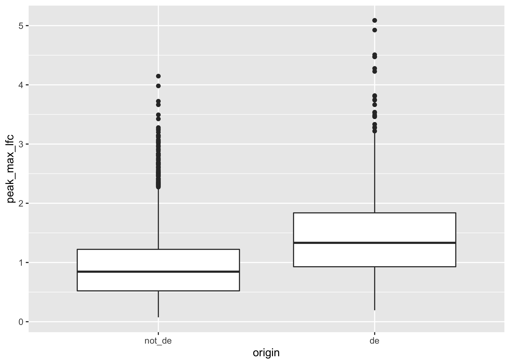
Figure 3.4: A boxplot of maximum LFCs for DA peaks for DE genes compared to non-DE genes where genes have at least one DA peak.
In general, the DE genes have larger maximum DA fold changes relative to the non-DE genes.
Next we examine how thresholds on the DA LFC modify the enrichment we observe of DA peaks near DE or non-DE genes. First, we want to know how the number of peaks within DE genes and non-DE genes change as we change threshold values on the peak LFC. As an example, we could compute this by arbitrarily chosen LFC thresholds of 1 or 2 as follows:
origin_peak_lfc <- genes_olap_peaks %>%
  group_by(origin) %>%
  summarize(
    peak_count = sum(!is.na(da_padj)) / n_distinct(resample),
    lfc1_peak_count =
      sum(abs(da_log2FC) > 1, na.rm=TRUE) / n_distinct(resample),
    lfc2_peak_count =
      sum(abs(da_log2FC) > 2, na.rm=TRUE) / n_distinct(resample)
  )
origin_peak_lfc
#> DataFrame with 2 rows and 4 columns
#> origin peak_count lfc1_peak_count lfc2_peak_count
#> <factor> <numeric> <numeric> <numeric>
#> 1 not_de 2391.8 369.5 32.5
#> 2 de 3416.0 1097.0 234.0Here we see that DE genes tend to have more DA peaks near them, and that the number of DA peaks decreases as we increase the DA LFC threshold (as expected). We now show how to compute the ratio of peak counts from DE compared to non-DE genes, so we can see how this ratio changes for various DA LFC thresholds.
For all variables except for the origin column we divide the first rows values by the second row, which will be the enrichment of peaks in DE genes compared to other genes. This requires us to reshape the summary table from long form back to wide form using the tidyr package. First we pivot the results of the peak_count columns into name-value pairs, then pivot again to place values into the origin column. Then we create a new column with the relative enrichment:
library(tidyr)
origin_peak_lfc %>%
  as.data.frame() %>%
  pivot_longer(cols = -origin) %>%
  pivot_wider(names_from = origin, values_from = value) %>%
  mutate(enrichment = de / not_de)
#> # A tibble: 3 x 4
#> name not_de de enrichment
#> <chr> <dbl> <dbl> <dbl>
#> 1 peak_count 2392. 3416 1.43
#> 2 lfc1_peak_count 370. 1097 2.97
#> 3 lfc2_peak_count 32.5 234 7.2The above table shows that relative enrichment increases for a larger LFC threshold.
Due to the one-to-many mappings of genes to peaks, it is unknown if we have the same number of DE genes participating or less, as we increase the threshold on the DA LFC. We can examine the number of genes with overlapping DA peaks at various thresholds by grouping and aggregating twice. First, the number of peaks that meet the thresholds are computed within each gene, origin, and resample group. Second, within the origin column, we compute the total number of peaks that meet the DA LFC threshold and the number of genes that have more than zero peaks (again averaging over the number of resamples).
genes_olap_peaks %>%
  group_by(gene_id, origin, resample) %>%
  reduce_ranges_directed(
    lfc1 = sum(abs(da_log2FC) > 1, na.rm=TRUE),
    lfc2 = sum(abs(da_log2FC) > 2, na.rm=TRUE)
  ) %>%
  group_by(origin) %>%
  summarize(
    lfc1_gene_count = sum(lfc1 > 0) / n_distinct(resample),
    lfc1_peak_count = sum(lfc1) / n_distinct(resample),
    lfc2_gene_count = sum(lfc2 > 0) / n_distinct(resample),
    lfc2_peak_count = sum(lfc2) / n_distinct(resample)
  )
#> DataFrame with 2 rows and 5 columns
#> origin lfc1_gene_count lfc1_peak_count lfc2_gene_count lfc2_peak_count
#> <factor> <numeric> <numeric> <numeric> <numeric>
#> 1 not_de 271.2 369.5 30.3 32.5
#> 2 de 515.0 1097.0 151.0 234.0To do this for many thresholds is cumbersome and would create a lot of
duplicate code. Instead we create a single function called
count_above_threshold() that accepts a variable and a vector of thresholds, and
computes the sum of the absolute value of the variable for each element in the
thresholds vector.
count_if_above_threshold <- function(var, thresholds) {
  lapply(thresholds, function(.) sum(abs(var) > ., na.rm = TRUE))
}
The above function will compute the counts for any arbitrary threshold, so we
can apply it over possible LFC thresholds of interest. We choose a grid of one
hundred thresholds based on the range of absolute LFC values in the da_peaks
GRanges object:
thresholds <- da_peaks %>%
  mutate(abs_lfc = abs(da_log2FC)) %>%
  with(
    seq(min(abs_lfc), max(abs_lfc), length.out = 100)
  )
The peak counts for each threshold are computed as a new list-column called value. First, the GRanges object has been grouped by the gene, origin, and the number of resamples columns. Then we aggregate over those columns, so each row will contain the peak counts for all of the thresholds for a gene, origin, and resample. We also maintain another list-column that contains the threshold values.
genes_peak_all_thresholds <- genes_olap_peaks %>%
  group_by(gene_id, origin, resample) %>%
  reduce_ranges_directed(
    value = count_if_above_threshold(da_log2FC, thresholds),
    threshold = list(thresholds)
  )
genes_peak_all_thresholds
#> GRanges object with 8239 ranges and 5 metadata columns:
#> seqnames ranges strand | gene_id origin
#> <Rle> <IRanges> <Rle> | <character> <factor>
#> [1] chr1 196641878-196661877 + | ENSG00000000971.15 de
#> [2] chr6 46119993-46139992 + | ENSG00000001561.6 de
#> [3] chr4 17567192-17587191 + | ENSG00000002549.12 de
#> [4] chr7 150790403-150810402 + | ENSG00000002933.8 de
#> [5] chr4 15768275-15788274 + | ENSG00000004468.12 de
#> ... ... ... ... . ... ...
#> [8235] chr17 43569620-43589619 - | ENSG00000175832.12 not_de
#> [8236] chr17 18250534-18270533 + | ENSG00000177427.12 not_de
#> [8237] chr20 63885182-63905181 + | ENSG00000101152.10 not_de
#> [8238] chr1 39071316-39091315 + | ENSG00000127603.25 not_de
#> [8239] chr8 41567187-41587186 + | ENSG00000158669.11 not_de
#> resample value threshold
#> <integer> <IntegerList> <NumericList>
#> [1] 0 1,1,1,... 0.0658243,0.1184840,0.1711436,...
#> [2] 0 1,1,1,... 0.0658243,0.1184840,0.1711436,...
#> [3] 0 6,6,6,... 0.0658243,0.1184840,0.1711436,...
#> [4] 0 4,4,4,... 0.0658243,0.1184840,0.1711436,...
#> [5] 0 11,11,11,... 0.0658243,0.1184840,0.1711436,...
#> ... ... ... ...
#> [8235] 10 1,1,1,... 0.0658243,0.1184840,0.1711436,...
#> [8236] 10 3,3,2,... 0.0658243,0.1184840,0.1711436,...
#> [8237] 10 5,5,5,... 0.0658243,0.1184840,0.1711436,...
#> [8238] 10 3,3,3,... 0.0658243,0.1184840,0.1711436,...
#> [8239] 10 3,3,3,... 0.0658243,0.1184840,0.1711436,...
#> -------
#> seqinfo: 25 sequences (1 circular) from hg38 genomeNow we can expand these list-columns into a long GRanges object using
expand_ranges(). This function will unlist the value and
threshold columns and lengthen the resulting GRanges object. To compute
the peak and gene counts for each threshold, we apply the same summarization as
before:
origin_peak_all_thresholds <- genes_peak_all_thresholds %>%
  expand_ranges() %>%
  group_by(origin, threshold) %>%
  summarize(
    gene_count = sum(value > 0) / n_distinct(resample),
    peak_count = sum(value) / n_distinct(resample)
  )
origin_peak_all_thresholds
#> DataFrame with 200 rows and 4 columns
#> origin threshold gene_count peak_count
#> <factor> <numeric> <numeric> <numeric>
#> 1 not_de 0.0658243 708.0 2391.4
#> 2 not_de 0.1184840 698.8 2320.6
#> 3 not_de 0.1711436 686.2 2178.6
#> 4 not_de 0.2238033 672.4 1989.4
#> 5 not_de 0.2764629 650.4 1785.8
#> ... ... ... ... ...
#> 196 de 5.06849 2 2
#> 197 de 5.12115 0 0
#> 198 de 5.17381 0 0
#> 199 de 5.22647 0 0
#> 200 de 5.27913 0 0Again we can compute the relative enrichment in LFCs in the same manner as before, by pivoting the results to long form then back to wide form to compute the enrichment.
origin_threshold_counts <- origin_peak_all_thresholds %>%
  as.data.frame() %>%
  pivot_longer(cols = -c(origin, threshold),
               names_to = c("type", "var"),
               names_sep = "_",
               values_to = "count") %>%
  select(-var)
We visualize the peak enrichment changes of DE genes relative to other genes as a line chart:
origin_threshold_counts %>%
  filter(type == "peak") %>%
  pivot_wider(names_from = origin, values_from = count) %>%
  mutate(enrichment =  de / not_de) %>%
  ggplot(aes(x = threshold, y = enrichment)) +
  geom_line() +
  labs(x = "logFC threshold", y = "Relative Enrichment")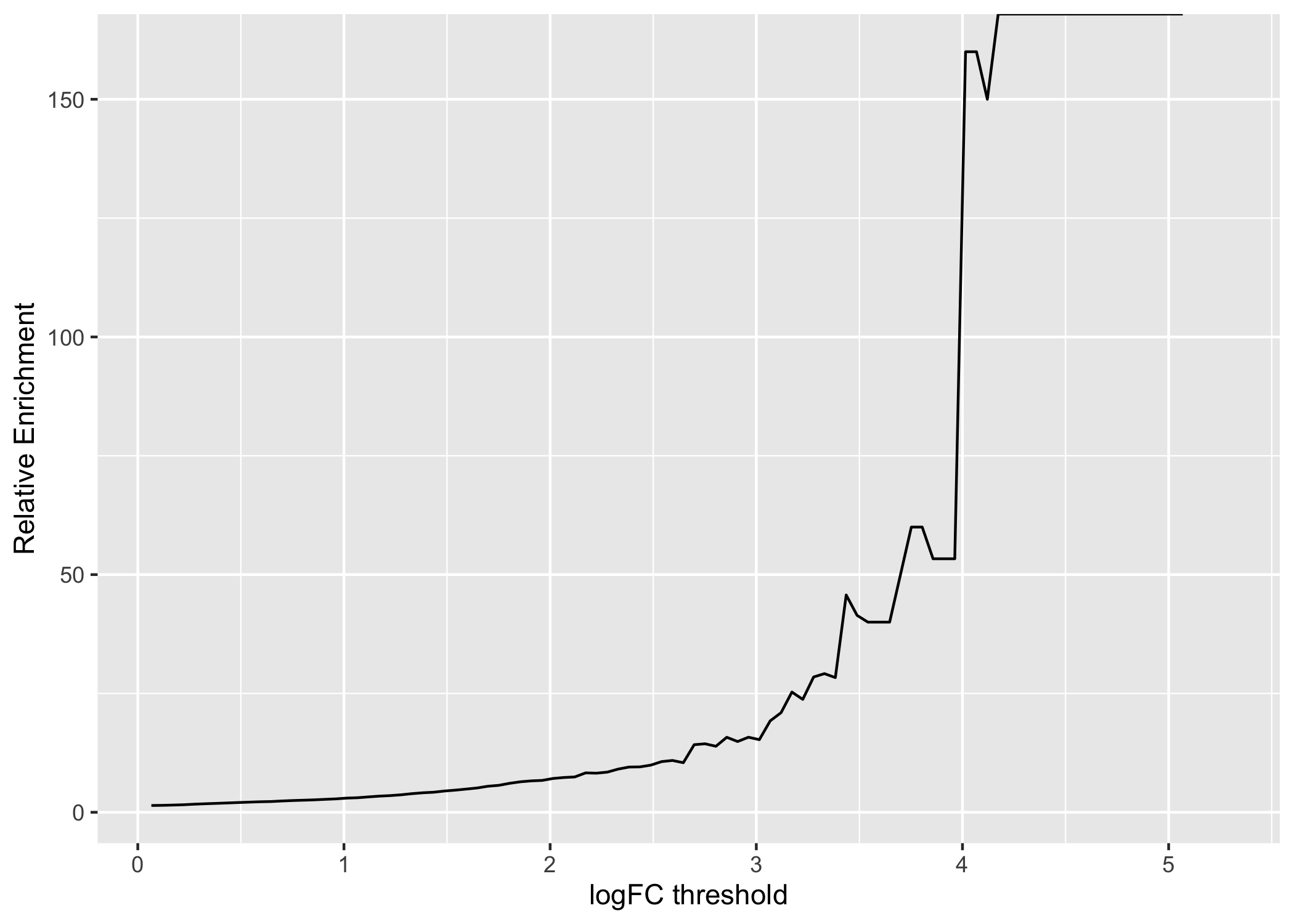
Figure 3.5: A line chart displaying how relative enrichment of DA peaks change between DE genes compared to non-DE genes as the absolute DA LFC threshold increases.
We computed the sum of DA peaks near the DE genes, for increasing LFC thresholds on the accessibility change. As we increased the threshold, the number of total peaks went down (likewise the mean number of DA peaks per gene). It is also likely the number of DE genes with a DA peak nearby with such a large change went down. We can investigate this with a plot that summarizes many of the aspects underlying the enrichment plot above.
origin_threshold_counts %>%
  ggplot(aes(x = threshold,
             y = count + 1,
             color = origin,
             linetype = type)) +
  geom_line() +
  scale_y_log10()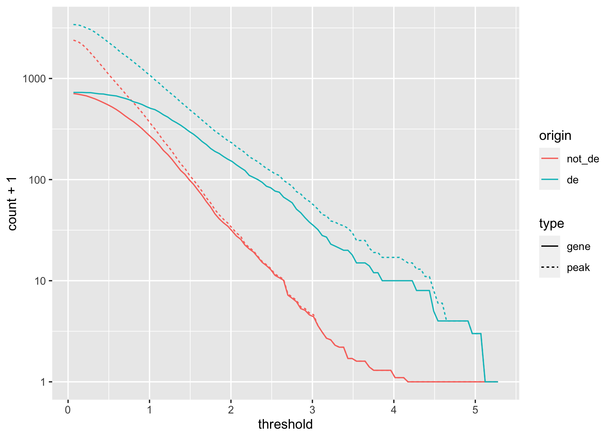
Figure 3.6: A line chart displaying how gene and peak counts change as the absolute DA LFC threshold increases. Lines are colored according to whether they represent a gene that is DE or not. Note the x-axis is on a \(log_{10}\) scale.