pdfsense: or understanding high dimensional parameter space
Source:vignettes/pdfsense.Rmd
pdfsense.RmdThis example is modified from the paper by Laa et al., here we show how we can use a tour to explore principal components space and any non-linear structure and clusters via non-linear embeddings.
Setting up the data
Data were obtained from CT14HERA2 parton distribution function fits as used in Laa et al., 2018. There are 28 directions in the parameter space of parton distribution function fit, each point in the variables labelled X1-X56 indicate moving +- 1 standard devation from the ‘best’ (maximum likelihood estimate) fit of the function. Each observation has all predictions of the corresponding measurement from an experiment. (see table 3 in that paper for more explicit details).
The remaining columns are:
- InFit: A flag indicating whether an observation entered the fit of CT14HERA2 parton distribution function
- Type: First number of ID
- ID: contains the identifier of experiment, 1XX/2XX/5XX correpsonds to Deep Inelastic Scattering (DIS) / Vector Boson Production (VBP) / Strong Interaction (JET). Every ID points to an experimental paper.
- pt: the per experiment observational id
- x,mu: the kinematics of a parton. x is the parton momentum fraction, and mu is the factorisation scale.
First, we take the data from a data.frame to a TourExperiment data structure:
library(SingleCellExperiment)
#> Loading required package: SummarizedExperiment
#> Loading required package: GenomicRanges
#> Loading required package: stats4
#> Loading required package: BiocGenerics
#> Loading required package: parallel
#>
#> Attaching package: 'BiocGenerics'
#> The following objects are masked from 'package:parallel':
#>
#>     clusterApply, clusterApplyLB, clusterCall, clusterEvalQ,
#>     clusterExport, clusterMap, parApply, parCapply, parLapply,
#>     parLapplyLB, parRapply, parSapply, parSapplyLB
#> The following objects are masked from 'package:stats':
#>
#>     IQR, mad, sd, var, xtabs
#> The following objects are masked from 'package:base':
#>
#>     anyDuplicated, append, as.data.frame, basename, cbind, colnames,
#>     dirname, do.call, duplicated, eval, evalq, Filter, Find, get, grep,
#>     grepl, intersect, is.unsorted, lapply, Map, mapply, match, mget,
#>     order, paste, pmax, pmax.int, pmin, pmin.int, Position, rank,
#>     rbind, Reduce, rownames, sapply, setdiff, sort, table, tapply,
#>     union, unique, unsplit, which, which.max, which.min
#> Loading required package: S4Vectors
#>
#> Attaching package: 'S4Vectors'
#> The following object is masked from 'package:base':
#>
#>     expand.grid
#> Loading required package: IRanges
#> Loading required package: GenomeInfoDb
#> Loading required package: Biobase
#> Welcome to Bioconductor
#>
#>     Vignettes contain introductory material; view with
#>     'browseVignettes()'. To cite Bioconductor, see
#>     'citation("Biobase")', and for packages 'citation("pkgname")'.
#> Loading required package: DelayedArray
#> Loading required package: matrixStats
#>
#> Attaching package: 'matrixStats'
#> The following objects are masked from 'package:Biobase':
#>
#>     anyMissing, rowMedians
#> Loading required package: BiocParallel
#>
#> Attaching package: 'DelayedArray'
#> The following objects are masked from 'package:matrixStats':
#>
#>     colMaxs, colMins, colRanges, rowMaxs, rowMins, rowRanges
#> The following objects are masked from 'package:base':
#>
#>     aperm, apply, rowsum
library(sneezy)
pdfsense <- TourExperiment(pdfsense, X1:X56)
pdfsense
#> class: TourExperiment
#> dim: 56 2808
#> metadata(0):
#> assays(1): view
#> rownames(56): X1 X2 ... X55 X56
#> rowData names(0):
#> colnames: NULL
#> colData names(6): InFit Type ... x mu
#> reducedDimNames(0):
#> spikeNames(0):
#> altExpNames(0):
#> neighborSetNames(0):
#> basisSetNames(0):
Linear embeddings and the tour
First we can estimate all nrow(pdfsense) principal components:
pdfsense <- embed_linear(pdfsense,
                         num_comp = nrow(pdfsense),
                         center = TRUE)
pdfsense
#> class: TourExperiment
#> dim: 56 2808
#> metadata(0):
#> assays(1): view
#> rownames(56): X1 X2 ... X55 X56
#> rowData names(0):
#> colnames: NULL
#> colData names(6): InFit Type ... x mu
#> reducedDimNames(1): pca_exact
#> spikeNames(0):
#> altExpNames(0):
#> neighborSetNames(0):
#> basisSetNames(0):
If we look at the data structure returned, we get a data structure called a LinearEmbeddingMatrix - which holds all the loadings and components.
pcs <- reducedDim(pdfsense, "pca_exact")
pcs
#> class: LinearEmbeddingMatrix
#> dim: 2808 56
#> metadata(0):
#> rownames: NULL
#> colnames(56): PC1 PC2 ... PC55 PC56
#> factorData names(1): sdev
Using this data structure, we can produce a screeplot:
factorData(pcs) <- cbind(
  factorData(pcs),
  variance_explained = factorData(pcs)$sdev / sum(factorData(pcs)$sdev),
  component = 1: nrow(factorData(pcs)),
  cumulative_var = cumsum(factorData(pcs)$sdev / sum(factorData(pcs)$sdev))
)

library(ggplot2)
ggplot(as.data.frame(factorData(pcs)),
       aes(x = component, y = variance_explained)) +
  geom_point() +
  labs(x = "Principal Component", y = "Proportion Variance Explained")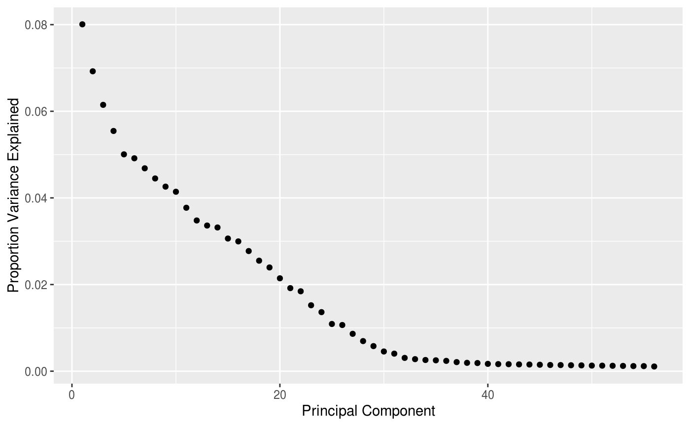
Approximately %70 of the variance in the pdf fits are explained by the first 15 principal components.
Next we can generate a set of bases to tour on the principal components. Note that we restrict our view to the first 6 principal components and generate 100 new bases via the grand tour (we choose 6 to follow the original paper):
pdfsense <- generate_bases(pdfsense,
                           .on = "pca_exact",
                           subset = 1:6)

dim(basisSet(pdfsense))
#> [1]   6   2 100
We can view a simple tour via sneezy_tour()
sneezy_tour(pdfsense)
#> Using half_range 0.83
#>
Frame 1 (1%)
Frame 2 (2%)
Frame 3 (3%)
Frame 4 (4%)
Frame 5 (5%)
Frame 6 (6%)
Frame 7 (7%)
Frame 8 (8%)
Frame 9 (9%)
Frame 10 (10%)
Frame 11 (11%)
Frame 12 (12%)
Frame 13 (13%)
Frame 14 (14%)
Frame 15 (15%)
Frame 16 (16%)
Frame 17 (17%)
Frame 18 (18%)
Frame 19 (19%)
Frame 20 (20%)
Frame 21 (21%)
Frame 22 (22%)
Frame 23 (23%)
Frame 24 (24%)
Frame 25 (25%)
Frame 26 (26%)
Frame 27 (27%)
Frame 28 (28%)
Frame 29 (29%)
Frame 30 (30%)
Frame 31 (31%)
Frame 32 (32%)
Frame 33 (33%)
Frame 34 (34%)
Frame 35 (35%)
Frame 36 (36%)
Frame 37 (37%)
Frame 38 (38%)
Frame 39 (39%)
Frame 40 (40%)
Frame 41 (41%)
Frame 42 (42%)
Frame 43 (43%)
Frame 44 (44%)
Frame 45 (45%)
Frame 46 (46%)
Frame 47 (47%)
Frame 48 (48%)
Frame 49 (49%)
Frame 50 (50%)
Frame 51 (51%)
Frame 52 (52%)
Frame 53 (53%)
Frame 54 (54%)
Frame 55 (55%)
Frame 56 (56%)
Frame 57 (57%)
Frame 58 (58%)
Frame 59 (59%)
Frame 60 (60%)
Frame 61 (61%)
Frame 62 (62%)
Frame 63 (63%)
Frame 64 (64%)
Frame 65 (65%)
Frame 66 (66%)
Frame 67 (67%)
Frame 68 (68%)
Frame 69 (69%)
Frame 70 (70%)
Frame 71 (71%)
Frame 72 (72%)
Frame 73 (73%)
Frame 74 (74%)
Frame 75 (75%)
Frame 76 (76%)
Frame 77 (77%)
Frame 78 (78%)
Frame 79 (79%)
Frame 80 (80%)
Frame 81 (81%)
Frame 82 (82%)
Frame 83 (83%)
Frame 84 (84%)
Frame 85 (85%)
Frame 86 (86%)
Frame 87 (87%)
Frame 88 (88%)
Frame 89 (89%)
Frame 90 (90%)
Frame 91 (91%)
Frame 92 (92%)
Frame 93 (93%)
Frame 94 (94%)
Frame 95 (95%)
Frame 96 (96%)
Frame 97 (97%)
Frame 98 (98%)
Frame 99 (99%)
Frame 100 (100%)
#> Finalizing encoding... done!
Alternatively, we can highlight an a grouping of interest, in this case the JET experiments:
highlight <-
  sneezy_tour(pdfsense,
              col = c("grey50", "darkred")[(colData(pdfsense)$Type == 5) + 1])
#> Using half_range 0.83
#>
Frame 1 (1%)
Frame 2 (2%)
Frame 3 (3%)
Frame 4 (4%)
Frame 5 (5%)
Frame 6 (6%)
Frame 7 (7%)
Frame 8 (8%)
Frame 9 (9%)
Frame 10 (10%)
Frame 11 (11%)
Frame 12 (12%)
Frame 13 (13%)
Frame 14 (14%)
Frame 15 (15%)
Frame 16 (16%)
Frame 17 (17%)
Frame 18 (18%)
Frame 19 (19%)
Frame 20 (20%)
Frame 21 (21%)
Frame 22 (22%)
Frame 23 (23%)
Frame 24 (24%)
Frame 25 (25%)
Frame 26 (26%)
Frame 27 (27%)
Frame 28 (28%)
Frame 29 (29%)
Frame 30 (30%)
Frame 31 (31%)
Frame 32 (32%)
Frame 33 (33%)
Frame 34 (34%)
Frame 35 (35%)
Frame 36 (36%)
Frame 37 (37%)
Frame 38 (38%)
Frame 39 (39%)
Frame 40 (40%)
Frame 41 (41%)
Frame 42 (42%)
Frame 43 (43%)
Frame 44 (44%)
Frame 45 (45%)
Frame 46 (46%)
Frame 47 (47%)
Frame 48 (48%)
Frame 49 (49%)
Frame 50 (50%)
Frame 51 (51%)
Frame 52 (52%)
Frame 53 (53%)
Frame 54 (54%)
Frame 55 (55%)
Frame 56 (56%)
Frame 57 (57%)
Frame 58 (58%)
Frame 59 (59%)
Frame 60 (60%)
Frame 61 (61%)
Frame 62 (62%)
Frame 63 (63%)
Frame 64 (64%)
Frame 65 (65%)
Frame 66 (66%)
Frame 67 (67%)
Frame 68 (68%)
Frame 69 (69%)
Frame 70 (70%)
Frame 71 (71%)
Frame 72 (72%)
Frame 73 (73%)
Frame 74 (74%)
Frame 75 (75%)
Frame 76 (76%)
Frame 77 (77%)
Frame 78 (78%)
Frame 79 (79%)
Frame 80 (80%)
Frame 81 (81%)
Frame 82 (82%)
Frame 83 (83%)
Frame 84 (84%)
Frame 85 (85%)
Frame 86 (86%)
Frame 87 (87%)
Frame 88 (88%)
Frame 89 (89%)
Frame 90 (90%)
Frame 91 (91%)
Frame 92 (92%)
Frame 93 (93%)
Frame 94 (94%)
Frame 95 (95%)
Frame 96 (96%)
Frame 97 (97%)
Frame 98 (98%)
Frame 99 (99%)
Frame 100 (100%)
#> Finalizing encoding... done!
highlight
Non-Linear embeddings
Now we can set up a non-linear embedding via t-SNE, here we use an approximate fit using a default perpelxity of 30.
set.seed(1999)
pdfsense <- embed_nonlinear(pdfsense, 2, .on = "pca_exact")
tsne <- reducedDim(pdfsense, "tsne_approx")
And we can use ggplot2 to construct a view of the embedding:
pl <- ggplot(
  data.frame(
    sampleFactors(tsne),
    colData(pdfsense)
  )) +
  geom_point(aes(x = Dim1, y = Dim2, col = factor(Type))) +
  scale_color_manual(values = c("blue", "orange", "darkred")) +
  labs(color = "Type") +
  theme_minimal() +
  theme(axis.text.x = element_blank(), axis.text.y = element_blank())
We can link a tour view next to the embedding to give us a clear picture of the clustering:
Next we can look at some diagnostics for the embedding, we can view the cluster centroids via a tour:
pdfsense <- estimate_neighbors(pdfsense, 30, .on = "tsne_approx")
pl +
  overlay_snn_centroids(sampleFactors(tsne)[,1],
                        sampleFactors(tsne)[,2],
                        neighborSet(pdfsense),
                        size = 5)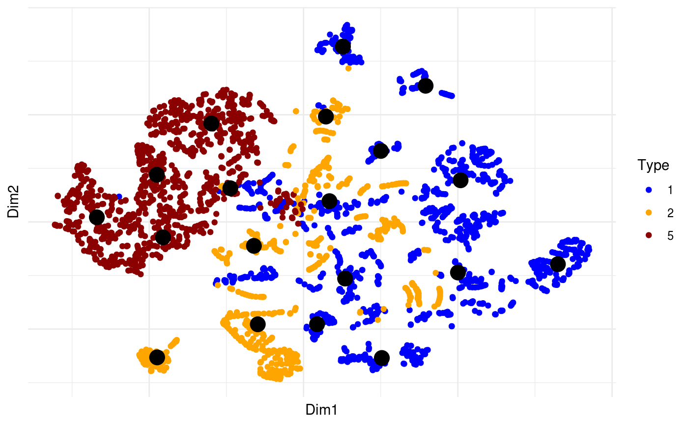
sneezy_centroids(pdfsense)
#> Using half_range 0.83
#>
Frame 1 (1%)
Frame 2 (2%)
Frame 3 (3%)
Frame 4 (4%)
Frame 5 (5%)
Frame 6 (6%)
Frame 7 (7%)
Frame 8 (8%)
Frame 9 (9%)
Frame 10 (10%)
Frame 11 (11%)
Frame 12 (12%)
Frame 13 (13%)
Frame 14 (14%)
Frame 15 (15%)
Frame 16 (16%)
Frame 17 (17%)
Frame 18 (18%)
Frame 19 (19%)
Frame 20 (20%)
Frame 21 (21%)
Frame 22 (22%)
Frame 23 (23%)
Frame 24 (24%)
Frame 25 (25%)
Frame 26 (26%)
Frame 27 (27%)
Frame 28 (28%)
Frame 29 (29%)
Frame 30 (30%)
Frame 31 (31%)
Frame 32 (32%)
Frame 33 (33%)
Frame 34 (34%)
Frame 35 (35%)
Frame 36 (36%)
Frame 37 (37%)
Frame 38 (38%)
Frame 39 (39%)
Frame 40 (40%)
Frame 41 (41%)
Frame 42 (42%)
Frame 43 (43%)
Frame 44 (44%)
Frame 45 (45%)
Frame 46 (46%)
Frame 47 (47%)
Frame 48 (48%)
Frame 49 (49%)
Frame 50 (50%)
Frame 51 (51%)
Frame 52 (52%)
Frame 53 (53%)
Frame 54 (54%)
Frame 55 (55%)
Frame 56 (56%)
Frame 57 (57%)
Frame 58 (58%)
Frame 59 (59%)
Frame 60 (60%)
Frame 61 (61%)
Frame 62 (62%)
Frame 63 (63%)
Frame 64 (64%)
Frame 65 (65%)
Frame 66 (66%)
Frame 67 (67%)
Frame 68 (68%)
Frame 69 (69%)
Frame 70 (70%)
Frame 71 (71%)
Frame 72 (72%)
Frame 73 (73%)
Frame 74 (74%)
Frame 75 (75%)
Frame 76 (76%)
Frame 77 (77%)
Frame 78 (78%)
Frame 79 (79%)
Frame 80 (80%)
Frame 81 (81%)
Frame 82 (82%)
Frame 83 (83%)
Frame 84 (84%)
Frame 85 (85%)
Frame 86 (86%)
Frame 87 (87%)
Frame 88 (88%)
Frame 89 (89%)
Frame 90 (90%)
Frame 91 (91%)
Frame 92 (92%)
Frame 93 (93%)
Frame 94 (94%)
Frame 95 (95%)
Frame 96 (96%)
Frame 97 (97%)
Frame 98 (98%)
Frame 99 (99%)
Frame 100 (100%)
#> Finalizing encoding... done!